Tutorial 3.2: Environmental Simulation
Part A: Into of Ladybug Tools
Ladybug Tools is an open-source suite of environmental analysis plugins for Grasshopper. It is the most widely used environmental simulation toolkit in computational design — adopted by firms like BIG, SOM, Arup, Perkins+Will, and taught at the AA, MIT, Harvard GSD, and many others. The project was started by Mostapha Sadeghipour Roudsari and has grown into a full ecosystem of interoperable tools.
The suite is named after pollinators. Each tool operates at a different scale and connects to different simulation engines:
| Tool | What it does | Simulation engine |
|---|---|---|
| Ladybug | Weather data visualization, sun path, wind rose, radiation analysis, shadow studies | Built-in |
| Honeybee | Building energy modeling, daylighting, glare, thermal comfort, HVAC sizing | EnergyPlus / OpenStudio, Radiance |
| Dragonfly | Urban-scale energy modeling, district analysis, urban heat island | URBANopt SDK |
| Butterfly | Computational fluid dynamics — wind flow, natural ventilation, pedestrian comfort | OpenFOAM |
These tools share data formats and form a pipeline: Ladybug reads the climate → Honeybee simulates building performance → Dragonfly scales to the city → Butterfly models airflow. For this course, we only use Ladybug — specifically its weather visualization and radiation analysis components.
🔗 ladybug.tools · Food4Rhino page · Ladybug Tools Forum
Weather Data and EPW Files
All environmental simulation in Ladybug starts with a weather file. The standard format is .epw (EnergyPlus Weather), which contains hourly measured data for an entire typical year — 8,760 values per data channel.
What's inside an EPW file:
| Data channel | Unit | Design relevance |
|---|---|---|
| Dry bulb temperature | °C | Thermal comfort, heating/cooling load |
| Relative humidity | % | Comfort, condensation risk |
| Wind speed | m/s | Natural ventilation, structural wind load |
| Wind direction | degrees from North | Facade exposure, ventilation inlet placement |
| Direct normal radiation | Wh/m² | Solar heat gain on surfaces facing the sun |
| Diffuse horizontal radiation | Wh/m² | Ambient sky light — relevant for all orientations |
| Global horizontal radiation | Wh/m² | Total solar energy on a flat surface |
Direct vs. diffuse radiation: Direct radiation is the beam from the sun — it casts sharp shadows and is strongest on surfaces facing the sun. Diffuse radiation is sunlight scattered by the atmosphere and clouds — it comes from the entire sky dome and affects all surfaces, even those in shadow. Together they define the total solar load on your building.
Where do EPW files come from? Weather stations around the world collect hourly measurements. These are compiled into "Typical Meteorological Year" (TMY) files — a synthetic year assembled from the most statistically representative months across decades of recorded data. This means the EPW file does not represent any single real year — it is an average composite. This is important: if you want to study climate change trends or analyze a specific extreme weather event, EPW/TMY data is not the right resource. It represents typical long-term conditions, not recent or future projections.
For Canadian locations, the dataset is called CWEC (Canadian Weather for Energy Calculations), maintained by Environment Canada.
EPW Map: Ladybug Tools hosts an interactive map of all available weather stations at ladybug.tools/epwmap. Each dot is a station. Click to copy the download URL directly into Grasshopper.
For this course we use: CAN_BC_Vancouver.Intl.AP.718920_CWEC2016.epw — the Vancouver International Airport station. This is the closest available station to UBC. When working on your own projects in the future, always check the EPW Map and choose the station nearest to your site — weather data can vary significantly even within a metropolitan area.
All data in an EPW file is in Celsius and metric units, regardless of your Rhino model units.
Installing Ladybug
Step 1: Go to Food4Rhino — Ladybug Tools and download the latest stable release.
Step 2: Unzip the downloaded file.
Step 3: Open the installer file inside the unzipped folder. Click the two toggle buttons in sequence to install. This may take 30 seconds or more as it downloads dependencies.
Step 4: Fully restart Rhino (not just close and reopen Grasshopper — restart the entire application).
Step 5: Open Grasshopper. You should see a new Ladybug tab in the component ribbon.
Update: if any installation issues occur, try the Pollination one-click installer: https://app.pollination.solutions/cad-plugins
Part B: Video Demo — Weather Visualization + Radiation Analysis
Download the Grasshopper file Getting_Started_With_Ladybug.gh and follow along with the video.
Make sure your Rhino file unit is set to meters! (in Rhino, run command "Units")
The demo covers the Ladybug pipeline:
- Importing weather data — downloading the Vancouver EPW file and reading it into Grasshopper
- Hourly Plot — annual heatmap of temperature (x = months, y = hours of day)
- Legend Parameters — controlling color ranges, segments, and formatting for readable charts
- Monthly Chart — aggregated daily/monthly bar charts using the Time Interval Operation
- Wind Rose — wind direction and speed frequency, seasonal filtering with Analysis Period
- Sun Path — solar trajectory diagram, analemmas, temperature overlay
- Direct Sun Hours — projecting sun vectors onto building surfaces to count sunlight hours per point
- Incident Radiation — full radiation analysis (kWh/m²) using Sky Matrix, accounting for both direct and diffuse radiation
The Food4Rhino download also includes example Grasshopper files demonstrating various Ladybug workflows. You are encouraged to explore these — they are a great way to learn additional analysis types beyond what we cover in class.
Additional Resources
- EPW Map — Ladybug Tools
- Ladybug Tools YouTube tutorials — comprehensive series covering weather data, sun paths, radiation, and more.
- Ladybug Tools Forum — active community for troubleshooting and advanced workflows.
Exercise 3.2
Using the UBC building massing, produce environmental analysis diagrams for the Alumni Centre facades and Lee Square, including surrounding vegetation as context geometry.
Required deliverables:
Site-level analysis (yearly):
- Wind Rose — annual wind direction and speed for Vancouver.
- Temperature chart — annual hourly plot or monthly chart of dry bulb temperature.
Sun studies (seasonal):
- Sun Path diagrams for three key dates: summer solstice (June 21), winter solstice (December 21), and equinox (March/September 21).
- Direct Sun Hours (Required)/ Shadow study (Optional) on the building facades for each of the same three dates — showing how sunlight and shadow change across seasons.
Representation:
- Play with your outputs: customize legends (color range, segments), try different parameters, and experiment with presentation quality. You can bake Ladybug geometries to Rhino and adjust colors, lineweights, and layer organization for cleaner screenshots.
- Add labels and annotations directly in Rhino using the
Textcommand — no need to export to another program for annotation.
An example submission is provided (using a different site, not UBC) to show the expected level of output.
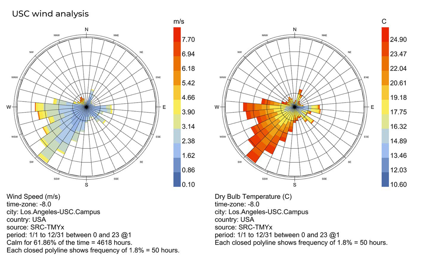
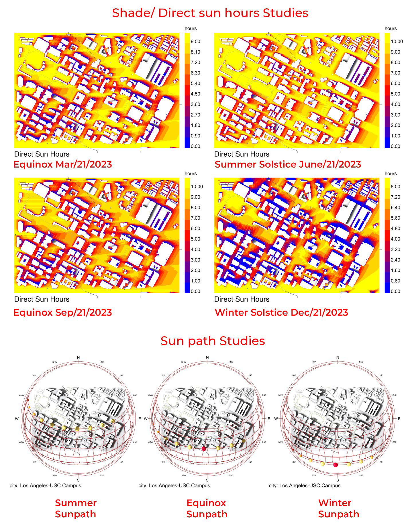
Note: the above shade analysis is directly done in Rhino, using command "Sun". Once you turn "on" the sun, you can manually set up the date and location. The shadow will show in "Rendered" mode.
Written observation (less than 150 words):
In your own words, describe what you found. What stands out about Vancouver's weather data? What did you observe about your specific site — which facades receive the most and least sun, how do shadows change across seasons, and what surprised you? This is not a formal essay — just a clear, concise summary of your environmental reading of the site.
Submit: Annotated screenshots + written observation.
Due: Mar 27 at 11:59 PM.