Tutorial 3.1: Spatial Data Injection

This tutorial covers how to bring real-world geographic data into Grasshopper — from downloading a map to generating a 3D urban model. The main tool is Caribou, a Grasshopper plugin for OpenStreetMap data.

Part 1: Basic Concepts (read)

What is GIS?

GIS (Geographic Information System) is a framework for managing, analyzing, and visualizing spatial data — data that is tied to a real location on Earth. For architects and urban designers, GIS is the primary way to access real-world site information: building footprints, street networks, topography, land use, zoning, population density, transit infrastructure, tree canopy coverage, and much more.

GIS has been a core tool in urban planning for decades. What has changed recently is that this data is now largely free, globally available, and increasingly easy to bring directly into 3D design environments like Rhino and Grasshopper.

Data Sources

OpenStreetMap (OSM) is a free, open-source, community-maintained global map. Anyone can contribute, and it is updated continuously. OSM covers buildings, roads, footpaths, waterways, parks, land use categories, and amenities (cafés, hospitals, transit stops, etc.) for virtually every location on Earth. Coverage and accuracy vary: dense urban areas like Vancouver and the UBC campus have excellent data, but building heights are often incomplete. Access through openstreetmap.org

Municipal and institutional datasets are more authoritative and precise, but limited to specific jurisdictions:

• UBC Campus Dataset — available via the UBC Library . Campus building footprints, infrastructure layers, and land use.
• Vancouver Open Data Portal → opendata.vancouver.ca — building footprints with height data, zoning boundaries, street network, tree inventory, permit records. Free download as Shapefile or GeoJSON.
• BC Data Catalogue → catalogue.data.gov.bc.ca — provincial datasets including terrain models, orthophotos, and administrative boundaries.

GIS software for viewing, filtering, and preparing data before bringing it into Grasshopper:

• ArcGIS (Esri) — industry standard in architecture and planning practice. Powerful but paid. ArcGIS Online has a free tier.
• QGIS — free, open-source, fully featured. Recommended for this course.
• For AI-assisted (text prompt to mapping) GIS scripting and querying, you can check the Vibe Coding for GIS tutorial.

File Types

GIS data comes in several formats. You will encounter these three most often:

Format	Extension	What it contains	How we use it
OSM / XML	.osm or .xml	OSM nodes, ways, relations, and all their metadata tags.	Downloaded from openstreetmap.org. Import into Grasshopper via plugins Caribou, Elk, Urbano, etc.
Shapefile	.shp + .dbf + .shx + .prj	Vector geometry + attribute table. Always a bundle of multiple files — keep them together.	Municipal datasets (Vancouver, UBC). Import into Grasshopper via “importSHP” component, or plugins such as @IT, GHSHP, etc.
GeoJSON	.geojson	Vector geometry + attributes in JSON format. Single file, human-readable.	Web maps, QGIS exports, open data APIs. Import into Grasshopper via plugin GeoJSON.

GIS Geometry: Points, Polylines, Polygons

All GIS data is 2D — it exists in a flat geographic coordinate plane. Every spatial feature is represented as one of three primitive geometry types:

• Points — a single coordinate location. Used for discrete objects: trees, bus stops, building entrances, fire hydrants, ATMs, streetlights.
• Polylines — a sequence of connected coordinates forming a line. Used for linear features: roads, footpaths, rivers, transit routes, property boundaries, contour lines.
• Polygons — a closed polyline enclosing an area. Used for area features: building footprints, parks, zoning lots, water bodies, land use zones, campus precincts.

In Grasshopper, OSM nodes become Points, ways become Polylines or closed Curves, and building footprints become closed planar curves ready to be extruded.

Attributes: Data Attached to Geometry

Every GIS feature carries an attribute table — a set of structured data fields attached to the geometry. A building polygon in OSM might have:

• name → "AMS Student Nest"
• building → university
• height → 28.5
• building:levels → 4

A road polyline might have:

• highway → primary
• name → "University Boulevard"
• maxspeed → 50
• lanes → 2

This is what makes GIS powerful for design. Geometry tells you where something is. Attributes tell you what it is and what it measures. The core operation in every GIS-to-3D workflow is: read the attribute, then use it to drive geometry. The most common example: extrude a building footprint polygon by its height attribute to generate a 3D building volume, which is automated in the plugin we will use.

Coordinate Systems (Optional)

GIS data is georeferenced — every coordinate corresponds to a real location on Earth. Two main systems are relevant here:

• Geographic coordinates (WGS84) — latitude and longitude in decimal degrees. Used by OSM, GPS, and most global datasets. Not in metres — distances are angular measures on the Earth's surface.
• Projected coordinates (e.g. UTM Zone 10N) — a flat 2D projection of the Earth's surface in metres. Used by Canadian municipal datasets and better suited for local measurement and analysis.

For this tutorial you don't need to manage this manually. Caribou converts OSM lat/long into Rhino world coordinates automatically when you parse the .xml file. In the future, if you are working with municipal Shapefiles via QGIS, export to UTM Zone 10N before bringing into Rhino for correct real-world scale.

 

Part 2: OSM to 3D Model with Caribou (practice)

Caribou (Philip Belesky) parses OpenStreetMap .xml files into Rhino geometry. Cross-platform (Windows + Mac), Rhino 6/7/8.

🔗 caribou.philipbelesky.com · Food4Rhino · YouTube tutorials (optional)

Caribou can be installed through package manager, Another plugin we will use UrbanXTool need manual installation.

Here is the Grasshopper script for reference:  Caribou_basics.gh

Watch and follow along this video demo:

 

Once you have created this workflow, save the Grasshopper file! For any other future site model, you only need to download the osm file and re-linked to the "file path".

Part 3 (Optional): Working with Other Data Types

Grasshopper scripts for workflows with shapefiles and spreadsheets are provided here for future reference.

GH Data Import.zip

Shapefiles — @IT: To import shapefiles and filter through attributes.

Excel / CSV — Bumblebee/Lunchbox :To import tabular non-spatial data (noise levels, pedestrian counts, program requirements)

 

Exercise 3.1:

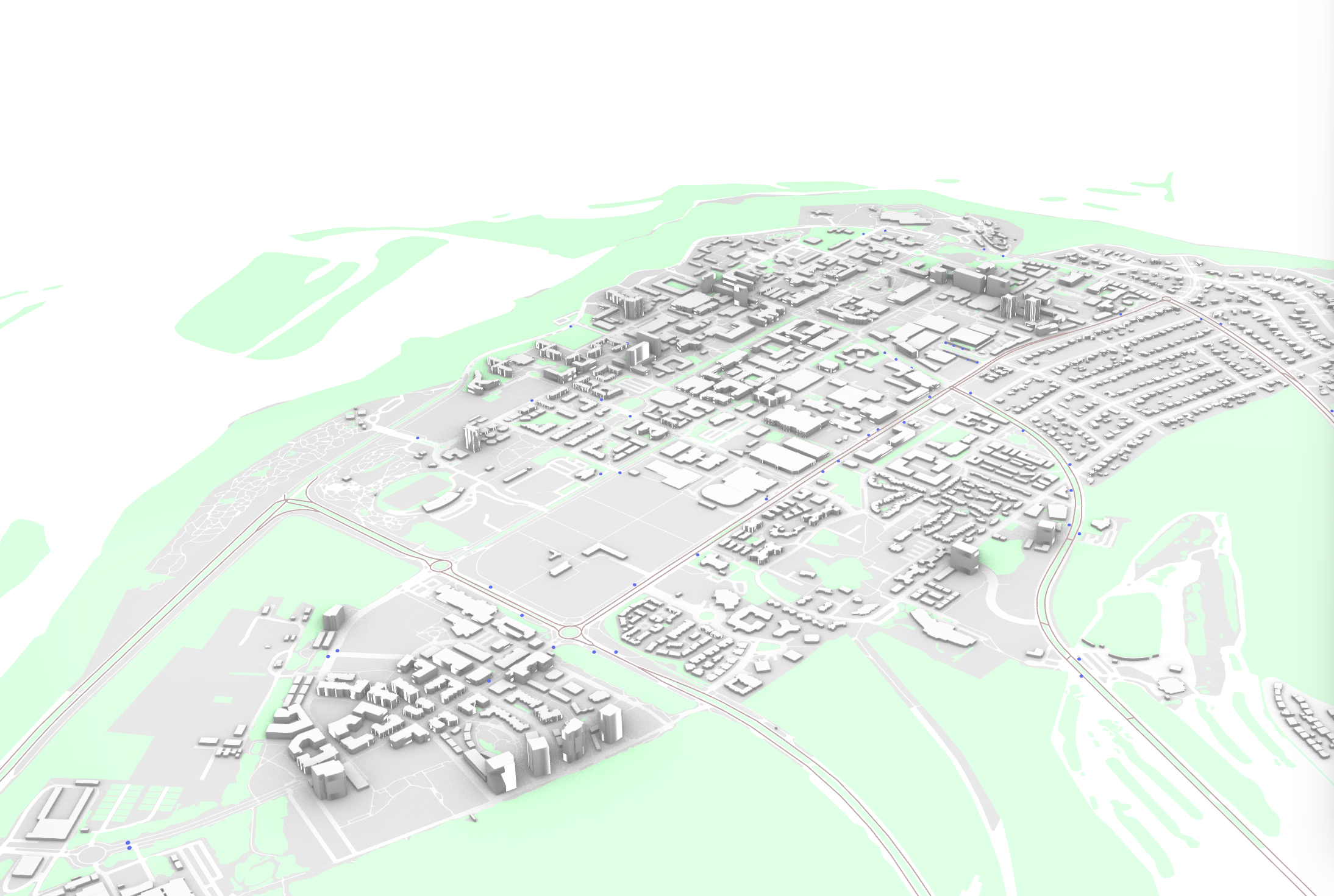
Model a minimum 500 × 500 m area of UBC campus centered on the Student Nest + Alumni Centre. 

Submit on Canvas by the following Friday, 11:59 PM:

Screenshot of your Rhino viewport — buildings extruded, parcel boundaries visible.

 

 

Common Issues

• Unit settings: Set Rhino Units to "meter" (use command Units in Rhino). This is the most common issue if streets are not offset correctly. After resetting the unit, middle-click the mouse to recompute Grasshopper, then click the "Zoom" button to view the geometry (it will scale down significantly)
• UrbanX Tool:
  • Mac users: Download version 3.0.0 instead of the latest version
  • Installation: Ensure the full folder (including all .dll files) is saved to the Grasshopper Components Folder
  • Processing time: The operation will take a long time to complete, so start with only the main road and fewer geometries. You can add more complexity later if successful. Keep the component disabled while testing—set your parameters and geometry first, then enable it.